Circuit models

We provide circuit models for the PDK elements, implemented using the sax circuit simulator. A dictionary with the available models can be obtained by running:

models = lnoi400.get_models()

These models are useful for constructing the scattering matrix of a building block, or of a hierarchical circuit. They are obtained by experimental characterization of the building blocks and with FDTD simulations, that provide the full wavelength-dependent behaviour. Since the lnoi400 PDK is conceived for optical C-band operation, the model results should not be trusted below 1500 or above 1600 nm.

Examples of circuit simulation using sax

import numpy as np
from functools import partial
import matplotlib.pyplot as plt
import gdsfactory as gf
import sax
import gplugins.sax as gs
import lnoi400

Circuit simulation of a splitter tree

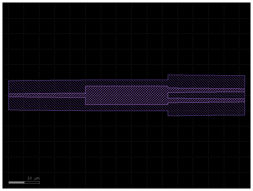
First, we display the circuit model of the 1x2 MMI shipped with the PDK.

splitter = gf.get_component("mmi1x2_optimized1550")
splitter.plot()

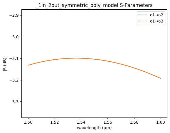
pcell_models = lnoi400.get_models()
mmi_model = pcell_models["mmi1x2_optimized1550"]
_ = gs.plot_model(
    mmi_model,
    wavelength_start=1.5,
    wavelength_stop=1.6,
    port1="o1",
    ports2=("o2", "o3"),
)

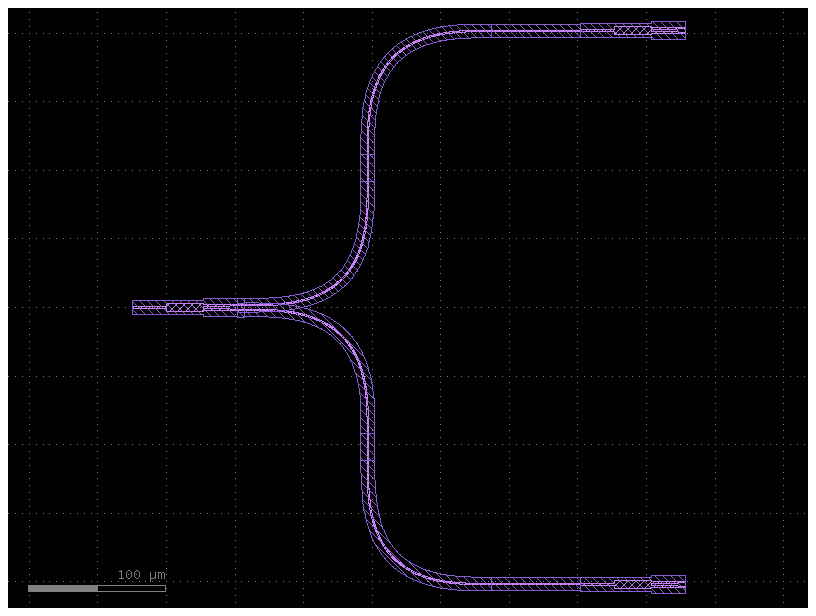
We then build a simple, two-level-deep splitter tree, creating a new gdsfactory hierarchical component.

@gf.cell
def splitter_chain(
    splitter = gf.get_component("mmi1x2_optimized1550"),
    column_offset = (250.0, 200.0),
    routing_reff = 90.0
) -> gf.Component:

    c = gf.Component()
    s0 = c << splitter
    s01 = c << splitter
    s02 = c << splitter
    s01.dmove(
        s01.ports["o1"].dcenter,
        s0.ports["o2"].dcenter + np.array(column_offset)
    )
    s02.dmove(
        s02.ports["o1"].dcenter,
        s0.ports["o3"].dcenter + np.array([column_offset[0], - column_offset[1]])
    )

    # Bend spec

    routing_bend = gf.get_component('L_turn_bend', radius=routing_reff)

    # Routing between splitters

    for ports_to_route in [
        (s0.ports["o2"], s01.ports["o1"]),
        (s0.ports["o3"], s02.ports["o1"]),
    ]:

        gf.routing.route_single(
            c,
            ports_to_route[0],
            ports_to_route[1],
            start_straight_length=5.0,
            end_straight_length=5.0,
            cross_section="xs_rwg1000",
            bend=routing_bend,
            straight="straight_rwg1000",
        )

    # Expose the I/O ports

    c.add_port(name="in", port=s0.ports["o1"])
    c.add_port(name="out_00", port=s01.ports["o2"])
    c.add_port(name="out_01", port=s01.ports["o3"])
    c.add_port(name="out_10", port=s02.ports["o2"])
    c.add_port(name="out_11", port=s02.ports["o3"])

    return c

chain = splitter_chain()
chain

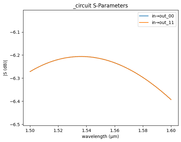
Let’s compile the circuit simulation using sax.

nl = chain.get_netlist()

models = {
    # The Euler bend should be sufficiently low-loss to be approximated with a straight waveguide
    # (if the frequency is not too low)
    "L_turn_bend": pcell_models["straight_rwg1000"],
    "straight_rwg1000": pcell_models["straight_rwg1000"],
    "mmi1x2_optimized1550": pcell_models["mmi1x2_optimized1550"],
}
circuit, _ = sax.circuit(netlist=nl, models=models)

_ = gs.plot_model(
    circuit,
    wavelength_start=1.5,
    wavelength_stop=1.6,
    port1="in",
    ports2=("out_00", "out_11"),
)

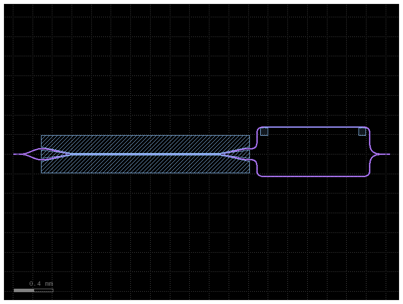
Simulation of a Mach-Zehnder interferometer with a thermo-optical phase shifter

First we take a look at the cell layout.

mzm_specs = dict(
    modulation_length=1500.0,
    with_heater=True,
    bias_tuning_section_length=1000.0,
)
mzm = gf.get_component(
    "mzm_unbalanced",
    **mzm_specs,
    )
mzm.plot()

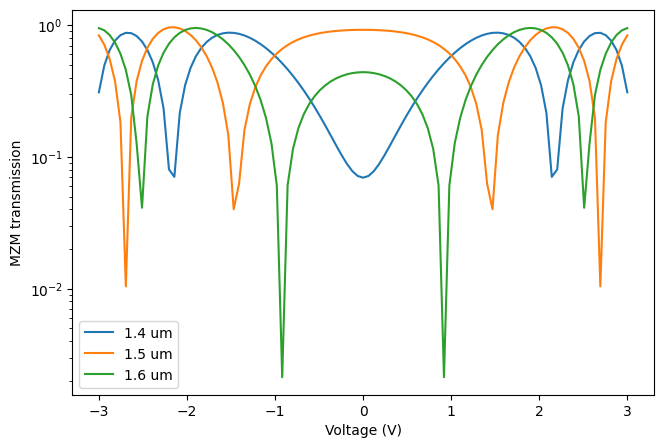
Then, we retrieve the circuit model and evaluate it for different wavelengths and voltages.

mzm_specs = dict(
    modulation_length=1500.0,
    heater_length=1000.0,
)
mzm_model = partial(
    pcell_models["mzm_unbalanced"],
    **mzm_specs,
)

fig = plt.figure(figsize=(7.5, 5))

wls = [1.4, 1.5, 1.6]
V_scan = np.linspace(-3, 3, 99)
for wl in wls:
    P_out = [np.abs(mzm_model(
        wl=wl,
        V_ht=V,
        )["o2", "o1"])
        for V in V_scan]
    plt.semilogy(V_scan, P_out, label=f'{wl} um')

plt.legend(loc='best')
plt.xlabel("Voltage (V)")
_ = plt.ylabel("MZM transmission")